A Quick Primer on Instrumental Variables

Author

Affiliation

Ian McCarthy, Emory University and NBER

Emory University, 2024

Outline

Assessing Selection on Unobservables
Basics of Instrumental Variables
Testing IV Assumptions
Interpreting IV Results
Common IV Designs Today

Assessing Selection on Unobservables

Say we estimate a regression like \[y_{i} = \delta D_{i} + \beta_{1} x_{1i} + \varepsilon_{i}\]
But we are concerned that the “true” specification is \[y_{i} = \delta D_{i} + \beta_{1} x_{1i} + \beta_{2} x_{2i} + \varepsilon_{i}\]
Idea: Extending the work of Altonji and others, Oster (2019) aims to decompose outome into a treatment effect (\(\delta\)), observed controls (\(x_{1}\)), unobserved controls (\(x_{2i}\)), and iid error

Oster (2019)

Key assumption: Selection on observables is informative about selection on unobservables

What is the maximum \(R^2\) value we could obtain if we observed \(x_{2}\)? Call this \(R_{\text{max}}^{2}\) (naturally bounded above by 1, but likely smaller)
What is the degree of selection on observed variables relative to unobserved variables? Denote the proportional relationship as \(\rho\) such that: \[\rho \times \frac{Cov(x_{1},D)}{Var(x_{1})} = \frac{Cov(x_{2},D)}{Var(x_{2})}.\]

Oster (2019)

Under an “equal relative contributions” assumption, we can write:

\[\delta^{*} \approx \hat{\delta}_{D,x_{1}} - \rho \times \left[\hat{\delta}_{D} - \hat{\delta}_{D,x_{1}}\right] \times \frac{R_{\text{max}}^{2} - R_{D,x_{1}}^{2}}{R_{D,x_{1}}^{2} - R_{x_{1}}^{2}} \xrightarrow{p} \delta.\]

Consider a range of \(R^{2}_{\text{max}}\) and \(\rho\) to bound the estimated treatment effect,

\[\left[ \hat{\delta}_{D,x_{1}}, \delta^{*}(\bar{R}^{2}_{max}, \rho) \right]\]

Augmented regression (somewhat out of place here)

Oster (2019) and similar papers can say something about how bad selection on unobservables would need to be
But what kind of “improvement” do we really get in practice?

Original test from Hausman (1978) not specific to endogeneity, just a general misspecification test
Compare estimates from one estimator (efficient under the null) to another estimator that is consistent but inefficient under the null
In IV context, also known as Durbin-Wu-Hausman test, due to the series of papers pre-dating Hausman (1978), including Durbin and Wu in the 1950s

Easily implemented as an “artificial” or “augmented” regression
We want to estimate \(y=\beta_{1}x_{1} + \beta_{2}x_{2} + \varepsilon\), with exogenous variables \(x_{1}\), endogenous variables \(x_{2}\), and instruments \(z\)
1. Regress each of the variables in \(x_{2}\) on \(x_{1}\) and \(z\) and form residuals, \(\hat{v}\), \(x_{2} = \lambda_{x} x_{1} + \lambda_{z} z + v\)
2. Include \(\hat{v}\) in the standard OLS regression of \(y\) on \(x_{1}\), \(x_{2}\), and \(\hat{v}\).
3. Test \(H_{0}: \beta_{\hat{v}} = 0\). Rejection implies OLS is inconsistent.

Intuition: Only way for \(x_{2}\) to be correlated with \(\varepsilon\) is through \(v\), assuming \(z\) is a “good” instrument

Summary

Do we have an endogeneity problem?
- Effects easily overcome by small selection on unobservables?
- Clear reverse causality problem?
What can we do about it?
- Matching, weighting, regression? Only for selection on observables
- DD, RD, differences in discontinuities? Specific designs and settings
- Instrumental variables?

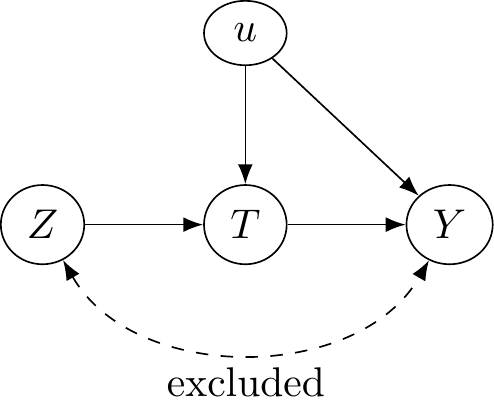
Instrumental Variables

What is instrumental variables

Instrumental Variables (IV) is a way to identify causal effects using variation in treatment particpation that is due to an exogenous variable that is only related to the outcome through treatment.

Simple example

\(y = \beta x + \varepsilon (x)\), where \(\varepsilon(x)\) reflects the dependence between our observed variable and the error term.
Simple OLS will yield \(\frac{dy}{dx} = \beta + \frac{d\varepsilon}{dx} \neq \beta\)

What does IV do?

The regression we want to do: \[y_{i} = \alpha + \delta D_{i} + \gamma A_{i} + \epsilon_{i},\] where \(D_{i}\) is treatment (think of schooling for now) and \(A_{i}\) is something like ability.
\(A_{i}\) is unobserved, so instead we run, \(y_{i} = \alpha + \beta D_{i} + \epsilon_{i}\)
From this “short” regression, we don’t actually estimate \(\delta\). Instead, we get an estimate of \[\beta = \delta + \lambda_{ds}\gamma \neq \delta,\] where \(\lambda_{ds}\) is the coefficient of a regression of \(A_{i}\) on \(D_{i}\).

Intuition

IV will recover the “long” regression without observing underlying ability

IF our IV satisfies all of the necessary assumptions.

More formally

We want to estimate \[E[Y_{i} | D_{i}=1] - E[Y_{i} | D_{i}=0]\]
With instrument \(Z_{i}\) that satisfies relevant assumptions, we can estimate this as \[E[Y_{i} | D_{i}=1] - E[Y_{i} | D_{i}=0] = \frac{E[Y_{i} | Z_{i}=1] - E[Y_{i} | Z_{i}=0]}{E[D_{i} | Z_{i}=1] - E[D_{i} | Z_{i}=0]}\]
In words, this is effect of the instrument on the outcome (“reduced form”) divided by the effect of the instrument on treatment (“first stage”)

Derivation

Recall “long” regression: \(Y=\alpha + \delta S + \gamma A + \epsilon\).

\[\begin{align} COV(Y,Z) & = E[YZ] - E[Y] E[Z] \\ & = E[(\alpha + \delta S + \gamma A + \epsilon)\times Z] - E[\alpha + \delta S + \gamma A + \epsilon)]E[Z] \\ & = \alpha E[Z] + \delta E[SZ] + \gamma E[AZ] + E[\epsilon Z] \\ & \hspace{.2in} - \alpha E[Z] - \delta E[S]E[Z] - \gamma E[A] E[Z] - E[\epsilon]E[Z] \\ & = \delta (E[SZ] - E[S] E[Z]) + \gamma (E[AZ] - E[A] E[Z]) \\ & \hspace{.2in} + E[\epsilon Z] - E[\epsilon] E[Z] \\ & = \delta C(S,Z) + \gamma C(A,Z) + C(\epsilon, Z) \end{align}\]

Derivation

Working from \(COV(Y,Z) = \delta COV(S,Z) + \gamma COV(A,Z) + COV(\epsilon,Z)\), we find

\[\delta = \frac{COV(Y,Z)}{COV(S,Z)}\]

if \(COV(A,Z)=COV(\epsilon, Z)=0\)

IVs in practice

Easy to think of in terms of randomized controlled trial…

Measure	Offered Seat	Not Offered Seat	Difference
Score	-0.003	-0.358	0.355
% Enrolled	0.787	0.046	0.741
Effect			0.48

Angrist et al., 2012. “Who Benefits from KIPP?” Journal of Policy Analysis and Management.

What is IV really doing

Think of IV as two-steps:

Isolate variation due to the instrument only (not due to endogenous stuff)
Estimate effect on outcome using only this source of variation

In regression terms

Interested in estimating \(\delta\) from \(y_{i} = \alpha + \beta x_{i} + \delta D_{i} + \varepsilon_{i}\), but \(D_{i}\) is endogenous (no pure “selection on observables”).

Step 1: With instrument \(Z_{i}\), we can regress \(D_{i}\) on \(Z_{i}\) and \(x_{i}\), \[D_{i} = \lambda + \theta Z_{i} + \kappa x_{i} + \nu,\] and form prediction \(\hat{D}_{i}\).

Step 2: Regress \(y_{i}\) on \(x_{i}\) and \(\hat{D}_{i}\), \[y_{i} = \alpha + \beta x_{i} + \delta \hat{D}_{i} + \xi_{i}\]

Derivation

Recall \(\hat{\theta}=\frac{C(Z,S)}{V(Z)}\), or \(\hat{\theta}V(Z) = C(S,Z)\). Then:

\[\begin{align} \hat{\delta} & = \frac{COV(Y,Z)}{COV(S,Z)} \\ & = \frac{\hat{\theta}C(Y,Z)}{\hat{\theta}C(S,Z)} = \frac{\hat{\theta}C(Y,Z)}{\hat{\theta}^{2}V(Z)} \\ & = \frac{C(\hat{\theta}Z,Y)}{V(\hat{\theta}Z)} = \frac{C(\hat{S},Y)}{V(\hat{S})} \end{align}\]

Animation for IV

R Code

df <- data.frame(Z = as.integer(1:200>100),
                 W = rnorm(200)) %>%
  mutate(X = .5+2*W +2*Z+ rnorm(200)) %>%
  mutate(Y = -X + 4*W + 1 + rnorm(200),time="1") %>%
  group_by(Z) %>%
  mutate(mean_X=mean(X),mean_Y=mean(Y),YL=NA,XL=NA) %>%
  ungroup()

#Calculate correlations
before_cor <- paste("1. Start with raw data. Correlation between X and Y: ",round(cor(df$X,df$Y),3),sep='')
afterlab <- '6. Draw a line between the points. The slope is the effect of X on Y.'

dffull <- rbind(
  #Step 1: Raw data only
  df %>% mutate(mean_X=NA,mean_Y=NA,time=before_cor),
  #Step 2: Add x-lines
  df %>% mutate(mean_Y=NA,time='2. Figure out what differences in X are explained by Z'),
  #Step 3: X de-meaned 
  df %>% mutate(X = mean_X,mean_Y=NA,time="3. Remove everything in X not explained by Z"),
  #Step 4: Remove X lines, add Y
  df %>% mutate(X = mean_X,mean_X=NA,time="4. Figure out what differences in Y are explained by Z"),
  #Step 5: Y de-meaned
  df %>% mutate(X = mean_X,Y = mean_Y,mean_X=NA,time="5. Remove everything in Y not explained by Z"),
  #Step 6: Raw demeaned data only
  df %>% mutate(X =  mean_X,Y =mean_Y,mean_X=NA,mean_Y=NA,YL=mean_Y,XL=mean_X,time=afterlab))

#Get line segments
endpts <- df %>%
  group_by(Z) %>%
  summarize(mean_X=mean(mean_X),mean_Y=mean(mean_Y))

p <- ggplot(dffull,aes(y=Y,x=X,color=as.factor(Z)))+geom_point()+
  geom_vline(aes(xintercept=mean_X,color=as.factor(Z)))+
  geom_hline(aes(yintercept=mean_Y,color=as.factor(Z)))+
  guides(color=guide_legend(title="Z"))+
  geom_segment(aes(x=ifelse(time==afterlab,endpts$mean_X[1],NA),
                   y=endpts$mean_Y[1],xend=endpts$mean_X[2],
                   yend=endpts$mean_Y[2]),size=1,color='blue')+
  scale_color_colorblind()+
  labs(title = 'The Relationship between Y and X, With Binary Z as an Instrumental Variable \n{next_state}')+
  transition_states(time,transition_length=c(6,16,6,16,6,6),state_length=c(50,22,12,22,12,50),wrap=FALSE)+
  ease_aes('sine-in-out')+
  exit_fade()+enter_fade()

animate(p,nframes=175)

Simulated data

n <- 5000
b.true <- 5.25
iv.dat <- tibble(
  z = rnorm(n,0,2),
  eps = rnorm(n,0,1),
  d = (z + 1.5*eps + rnorm(n,0,1) >0.25),
  y = 2.5 + b.true*d + eps + rnorm(n,0,0.5)
)

endogenous eps: affects treatment and outcome
z is an instrument: affects treatment but no direct effect on outcome

Results with simulated data

Recall that the true treatment effect is 5.25


Call:
lm(formula = y ~ d, data = iv.dat)

Residuals:
    Min      1Q  Median      3Q     Max 
-3.6842 -0.6864 -0.0033  0.6899  4.3910 

Coefficients:
            Estimate Std. Error t value Pr(>|t|)    
(Intercept)  2.08624    0.01986   105.1   <2e-16 ***
dTRUE        6.15766    0.02915   211.2   <2e-16 ***
---
Signif. codes:  0 '***' 0.001 '**' 0.01 '*' 0.05 '.' 0.1 ' ' 1

Residual standard error: 1.028 on 4998 degrees of freedom
Multiple R-squared:  0.8993,    Adjusted R-squared:  0.8992 
F-statistic: 4.462e+04 on 1 and 4998 DF,  p-value: < 2.2e-16

TSLS estimation - Dep. Var.: y
                  Endo.    : d
                  Instr.   : z
Second stage: Dep. Var.: y
Observations: 5,000
Standard-errors: IID 
            Estimate Std. Error t value  Pr(>|t|)    
(Intercept)  2.50612   0.029812 84.0643 < 2.2e-16 ***
fit_dTRUE    5.25274   0.054380 96.5941 < 2.2e-16 ***
---
Signif. codes:  0 '***' 0.001 '**' 0.01 '*' 0.05 '.' 0.1 ' ' 1
RMSE: 1.12249   Adj. R2: 0.879822
F-test (1st stage), dTRUE: stat = 2,606.7, p < 2.2e-16, on 1 and 4,998 DoF.
               Wu-Hausman: stat =   558.7, p < 2.2e-16, on 1 and 4,997 DoF.

Two-stage equivalence

R Code

step1 <- lm(d ~ z, data=iv.dat)
d.hat <- predict(step1)
step2 <- lm(y ~ d.hat, data=iv.dat)
summary(step2)


Call:
lm(formula = y ~ d.hat, data = iv.dat)

Residuals:
    Min      1Q  Median      3Q     Max 
-8.2540 -2.1816 -0.1687  2.2333 10.7230 

Coefficients:
            Estimate Std. Error t value Pr(>|t|)    
(Intercept)  2.50612    0.07575   33.09   <2e-16 ***
d.hat        5.25274    0.13817   38.02   <2e-16 ***
---
Signif. codes:  0 '***' 0.001 '**' 0.01 '*' 0.05 '.' 0.1 ' ' 1

Residual standard error: 2.853 on 4998 degrees of freedom
Multiple R-squared:  0.2243,    Adjusted R-squared:  0.2242 
F-statistic:  1445 on 1 and 4998 DF,  p-value: < 2.2e-16

Assumptions of IV

Key IV assumptions

Exclusion: Instrument is uncorrelated with the error term
Validity: Instrument is correlated with the endogenous variable
Monotonicity: Treatment more (less) likely for those with higher (lower) values of the instrument

Assumptions 1 and 2 sometimes grouped into an only through condition.

Checking instrument

Bare minimum (probably not even that) is to check first stage and reduced form:

Check the ‘first stage’


Call:
lm(formula = d ~ z, data = iv.dat)

Residuals:
     Min       1Q   Median       3Q      Max 
-1.06484 -0.33153 -0.02397  0.34092  1.40327 

Coefficients:
            Estimate Std. Error t value Pr(>|t|)    
(Intercept) 0.462255   0.005719   80.83   <2e-16 ***
z           0.144829   0.002837   51.06   <2e-16 ***
---
Signif. codes:  0 '***' 0.001 '**' 0.01 '*' 0.05 '.' 0.1 ' ' 1

Residual standard error: 0.4044 on 4998 degrees of freedom
Multiple R-squared:  0.3428,    Adjusted R-squared:  0.3426 
F-statistic:  2607 on 1 and 4998 DF,  p-value: < 2.2e-16

Check the ‘reduced form’


Call:
lm(formula = y ~ z, data = iv.dat)

Residuals:
    Min      1Q  Median      3Q     Max 
-8.2540 -2.1816 -0.1687  2.2333 10.7230 

Coefficients:
            Estimate Std. Error t value Pr(>|t|)    
(Intercept)  4.93423    0.04034  122.31   <2e-16 ***
z            0.76075    0.02001   38.02   <2e-16 ***
---
Signif. codes:  0 '***' 0.001 '**' 0.01 '*' 0.05 '.' 0.1 ' ' 1

Residual standard error: 2.853 on 4998 degrees of freedom
Multiple R-squared:  0.2243,    Adjusted R-squared:  0.2242 
F-statistic:  1445 on 1 and 4998 DF,  p-value: < 2.2e-16

Do we need IV?

Let’s run an “augmented regression” to see if our OLS results are sufficiently different than IV

R Code

d.iv <- lm(d ~ z, data=iv.dat)
d.resid <- residuals(d.iv)
haus.test <- lm(y ~ d + d.resid, data=iv.dat)
summary(haus.test)


Call:
lm(formula = y ~ d + d.resid, data = iv.dat)

Residuals:
    Min      1Q  Median      3Q     Max 
-3.3708 -0.6429 -0.0112  0.6636  4.1932 

Coefficients:
            Estimate Std. Error t value Pr(>|t|)    
(Intercept)  2.50612    0.02589   96.80   <2e-16 ***
dTRUE        5.25274    0.04723  111.22   <2e-16 ***
d.resid      1.37689    0.05825   23.64   <2e-16 ***
---
Signif. codes:  0 '***' 0.001 '**' 0.01 '*' 0.05 '.' 0.1 ' ' 1

Residual standard error: 0.975 on 4997 degrees of freedom
Multiple R-squared:  0.9094,    Adjusted R-squared:  0.9094 
F-statistic: 2.508e+04 on 2 and 4997 DF,  p-value: < 2.2e-16

Test for significance of d.resid suggests OLS is inconsistent in this case

Testing exclusion

Exclusion restriction says that your instrument does not directly affect your outcome
Potential testing ideas:
- “zero-first-stage” (subsample on which you know the instrument does not affect the endogenous variable)
- augmented regression of reduced-form effect with subset of instruments (overidentified models only)
- Sargan or Hansen’s J test (null hypothesis is that instruments are uncorrelated with residuals)

Kippersluis and Rietveld (2018), “Beyond Plausibly Exogenous”

“zero-first-stage” test
Focus on subsample for which your instrument is not correlated with the endogenous variable of interest
1. Regress the outcome on all covariates and the instruments among this subsample
2. Coefficient on the instruments captures any potential direct effect of the instruments on the outcome (since the correlation with the endogenous variable is 0 by assumption).

Beckert (2020), “A Note on Specification Testing…”

With at least \(n\) valid instruments, test if all instruments are valid against the alternative that up to \(m - n\) instruments are valid
1. Estimate the first-stage regressions and save residuals, denoted \(\hat{u}\).
2. Estimate the “artificial” regression \[y=\beta x + \delta \tilde{z} + \gamma \hat{u} + \varepsilon\] where \(\tilde{z}\) denotes a subset of \(m-n\) instruments from the full instrument matrix \(z\).
3. Test the null that \(\delta=0\) using a standard F-test

Solving an Exclusion Problem

Conley, Hansen, and Rossi (2012) and “plausible exogeneity”, union of confidence intervals approach:

Suppose extent of violation is known in \(y_{i} = \beta x_{i} + \gamma z_{i} + \varepsilon_{i}\), so that \(\gamma = \gamma_{0}\)
IV/TSLS applied to \(y_{i} - \gamma_{0}z_{i} = \beta x_{i} + \varepsilon_{i}\) works
With \(\gamma_{0}\) unknown…do this a bunch of times!
- Pick \(\gamma=\gamma^{b}\) for \(b=1,...,B\)
- Obtain \((1-\alpha)\) % confidence interval for \(\beta\), denoted \(CI^{b}(1-\alpha)\)
- Compute final CI as the union of all \(CI^{b}\)

Solving an Exclusion Problem

Nevo and Rosen (2012):

\[y_{i} = \beta x_{i} + \delta D_{i} + \varepsilon_{i}\]

Allow instrument, \(z\), to be correlated with \(\varepsilon\), but \(|\rho_{x, \varepsilon}| \geq |\rho_{z, \varepsilon}|\)
i.e., IV is better than just using the endogenous variable
Assume \(\rho_{x, \varepsilon} \times \rho_{z, \varepsilon} >0\) (same sign of correlation in the error)
Denote \(\lambda = \frac{\rho_{z, \varepsilon}}{\rho_{x, \varepsilon}}\), then valid \(IV\) would be \(V(z) = \sigma_{x} z - \lambda \sigma_{z} x\)
Can bound \(\beta\) using range of \(\lambda\)

Instrument Validity

Just says that your instrument is correlated with the endogenous variable, but what about the strength of the correlation?

Why we care about instrument strength

Recall our schooling and wages equation, \[y = \beta S + \epsilon.\] Bias in IV can be represented as:

\[Bias_{IV} \approx \frac{Cov(S, \epsilon)}{V(S)} \frac{1}{F+1} = Bias_{OLS} \frac{1}{F+1}\]

Bias in IV may be close to OLS, depending on instrument strength
Bigger problem: Bias could be bigger than OLS if exclusion restriction not fully satisfied

Testing strength of instruments

Two things going on simultaneously:

Strength of the first-stage
Inference on coefficient of interest in the structural equation

Applied researchers tend to (wrongly) think of these as separate issues.

References

Aizer, Anna, and Joseph J. Doyle Jr. 2015. “Juvenile Incarceration, Human Capital, and Future Crime: Evidence from Randomly Assigned Judges *.” The Quarterly Journal of Economics 130 (2): 759–803. https://doi.org/10.1093/qje/qjv003.
Autor, David H., David Dorn, and Gordon H. Hanson. 2013. “The China Syndrome: Local Labor Market Effects of Import Competition in the United States.” American Economic Review 103 (6): 2121–68. https://doi.org/10.1257/aer.103.6.2121.
Beckert, Walter. 2020. “A Note on Specification Testing in Some Structural Regression Models.” Oxford Bulletin of Economics and Statistics 82 (3): 686–95.
Borusyak, Kirill, and Peter Hull. 2023. “Nonrandom Exposure to Exogenous Shocks.” Econometrica 91 (6): 2155–85. https://doi.org/10.3982/ECTA19367.
Borusyak, Kirill, Peter Hull, and Xavier Jaravel. 2021. “Quasi-Experimental Shift-Share Research Designs.” Review of Economic Studies.
Conley, Timothy G, Christian B Hansen, and Peter E Rossi. 2012. “Plausibly Exogenous.” Review of Economics and Statistics 94 (1): 260–72.
Goldsmith-Pinkham, Paul, Isaac Sorkin, and Henry Swift. 2020. “Bartik Instruments: What, When, Why, and How.” American Economic Review 110 (8): 2586–2624. https://doi.org/10.1257/aer.20181047.
Kippersluis, Hans van, and Cornelius A Rietveld. 2018. “Beyond Plausibly Exogenous.” The Econometrics Journal 21 (3): 316–31.
Kleibergen, Frank, and Richard Paap. 2006. “Generalized Reduced Rank Tests Using the Singular Value Decomposition.” Journal of Econometrics 133 (1): 97–126.
Lee, David S., Justin McCrary, Marcelo J. Moreira, and Jack R. Porter. 2021. “Valid t-Ratio Inference for IV.” Working {Paper}. Working Paper Series. National Bureau of Economic Research. https://doi.org/10.3386/w29124.
Moreira, Marcelo J. 2003. “A Conditional Likelihood Ratio Test for Structural Models.” Econometrica 71 (4): 1027–48. https://doi.org/10.1111/1468-0262.00438.
Nevo, Aviv, and Adam M Rosen. 2012. “Identification with Imperfect Instruments.” Review of Economics and Statistics 94 (3): 659–71.
Olea, José Luis Montiel, and Carolin Pflueger. 2013. “A Robust Test for Weak Instruments.” Journal of Business & Economic Statistics 31 (3): 358–69.
Oster, Emily. 2019. “Unobservable Selection and Coefficient Stability: Theory and Evidence.” Journal of Business & Economic Statistics 37 (2): 187–204. https://doi.org/10.1080/07350015.2016.1227711.
Sanderson, Eleanor, and Frank Windmeijer. 2016. “A Weak Instrument F-Test in Linear IV Models with Multiple Endogenous Variables.” Journal of Econometrics 190 (2): 212–21.
Stock, James H, and Motohiro Yogo. 2005. “Testing for Weak Instruments in Linear IV Regression.” In Identification and Inference for Econometric Models: Essays in Honor of Thomas Rothenberg. Cambridge University Press.